EVIEWS操作各种模型学习.docx

EVIEWS操作各种模型学习.docx

《EVIEWS操作各种模型学习.docx》由会员分享，可在线阅读，更多相关《EVIEWS操作各种模型学习.docx（58页珍藏版）》请在冰点文库上搜索。

EVIEWS操作各种模型学习

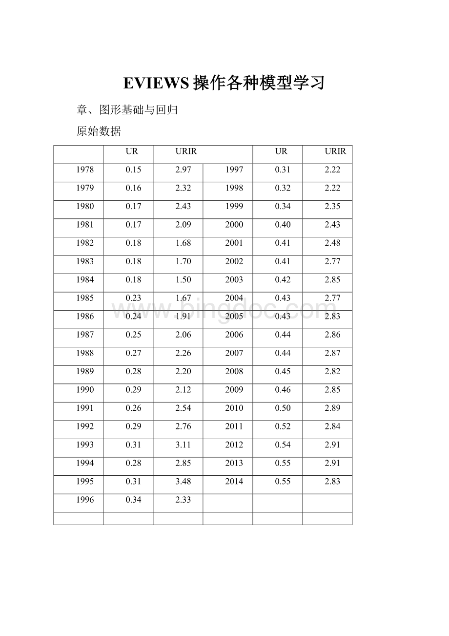
章、图形基础与回归

原始数据

UR

URIR

UR

URIR

1978

0.15

2.97

1997

0.31

2.22

1979

0.16

2.32

1998

0.32

2.22

1980

0.17

2.43

1999

0.34

2.35

1981

0.17

2.09

2000

0.40

2.43

1982

0.18

1.68

2001

0.41

2.48

1983

0.18

1.70

2002

0.41

2.77

1984

0.18

1.50

2003

0.42

2.85

1985

0.23

1.67

2004

0.43

2.77

1986

0.24

1.91

2005

0.43

2.83

1987

0.25

2.06

2006

0.44

2.86

1988

0.27

2.26

2007

0.44

2.87

1989

0.28

2.20

2008

0.45

2.82

1990

0.29

2.12

2009

0.46

2.85

1991

0.26

2.54

2010

0.50

2.89

1992

0.29

2.76

2011

0.52

2.84

1993

0.31

3.11

2012

0.54

2.91

1994

0.28

2.85

2013

0.55

2.91

1995

0.31

3.48

2014

0.55

2.83

1996

0.34

2.33

UR

-raESZ一os①三ueno

76543210

-PULIONjoSQsueno

URIR

:

、分布图：

JB〉3判断为正太分布

S是偏度

K是峰度

5-t

Series:

UR

Sample137

4-

Observations37

3-

2-

MeanMedianMaximumMinimumStd.Dev.

SkewnessKurtosis

0.336145

0.312400

0.547000

0.15087-

0.120626

0.143256

1.887565

Jarque-Bera2.034384

Probability0.361609

0.2

0.3

0.4

0.5

三、UR的单因素联表

TabulationofUR

Date:

09/05/15Time:

21:

25

Sample:

137

Ineludedobservations:

37

Numberofcategories:

5

Value

Count

Percent

Cumulative

Count

Cumulative

Percent

[0.1,0.2）

7

18.92

7

18.92

[0.2,0.3）

9

24.32

16

43.24

[0.3,0.4）

6

16.22

22

59.46

[0.4,0.5）

11

29.73

33

89.19

[0.5,0.6）

4

10.81

37

100.00

Total

37

100.00

37

100.00

四、协方差与相矢丫生

CovarianeeAnalysis:

Ordinary

Date:

09/05/15Time:

21:

40

Sample:

137

Ineludedobservations:

37

Covarianee

Correlation

UR

URIR

UR

0.014157

1.000000

URIR

0.033170

0.204852

0.615934

1.000000

Date:

09/05/15Time:

21:

44

Sample:

137

Ineludedobservations:

37

Correlationsareasymptoticallyconsistentapproximations

URrURIR（-i）

UR,URIR（+i>

Oi

Oi□i

匚匸匚匚匸匚匚

lag

lead

0

0.6159

0.&159

1

0.5767

0.6549

2

0.4997

0.6515

3

0.4282

0.6384

4

0.3795

0.5755

5

0.3621

0.4990

6

0.3267

0.4159

7

0.3292

0.2918

8

0.2983

0.1732

9

0.2585

0.0795

10

0.1997

0.0124

11

0.1420

-0.0556

12

□0809

-0.0998

13

0.0097

-0.1538

14

-0.0231

■0.1740

15

-0.033B

-0.1790

16

-0.0565

*0.1401

17

-0.0433

-0.1238

18

-0.0316

-0.0532

19

-0.0395

-0.0939

20

-0.1629

-0.1381

1.0

0.8

0.6

0.4

0.2

0.0

1.0

0.8

0.6

0.4

0.2

0.0

五、CDF经验分布图

URIR

UR

图

QQ-亠'八

UR

QuantilesofUR

URIR

6

I

.2

■

.3

I

.4

I.5

.6

QuantilesofURIR

84

22

o

2

6

2

6

3

4

2

2

3o

2

1—

1-

七、回归散点图

UR

邻近拟合散点图：

（分布回归的结

果）

3.6

$O

八、实际值、拟合值、残差值折线图

九、回归模型预测

URF—±2S.E

Forecast:

URF

Actual:

UR

Forecastsample:

137

Ineludedobservations:

37

RootMeanSquaredError0.093736

MeanAbsoluteError0.072711

MeanAbs.PercentError25.93140

TheilInequalityCoefficientO.133790

BiasProportion0.000000

VarianeeProportion0.237674

CovarianeeProportion0.762326

十、两回归系数的联合检验置信区间是一个椭圆区域

!

八一、Wald系数约束条件检验

WaldTest:

Equation:

Untitled

RestrictionsarelinearincgeAI匚ients

TestStatistic

Value

df

Probability

F-statisticChi-square

272.1503

（1.35）

0.0000

272.1503

1

0.0000

NullHypothesisSummary:

NormalizedRestriction[=Q）

Value

Std.Err,

-1+C

（1）+C

（2）

-0,907527

0.055012

Chow分割点检验结果

ChowBreakpointTest1991

NullHypothesis:

Nobreaksatspecifiedbreakpoints

Varyingregressors:

AllequationvariablesEquationSample:

19782014

F'Statistic

11.00551

Prob.F（2r33）

0.0002

Loglikelihoodratio

18.90797

ProbJChi-Square

（2）

0.0001

WaldStatistic

22.01103

Prob.Chi-Squa（e

（2）

0.0000

F、LR的P值显著，表示：

模型无显著的结构变化

十二、Chow稳定性检验（p75）

Chow预测结果：

ChowForecastTest:

Forecastfrom1991to2014

F-statistic

Loglikelihoodratio

4.744782

89.83840

PfOb.F（24,11）

Prob.Chi-Square（24）

0.0050

0.0000

TestEquation:

DependentVariable:

URMethod:

LeastSquares

Date:

09/07/15Time:

10:

31

Sample:

197S1990

Ineluded!

observations:

13

Coefficient

Std.Errort-Statistic

Prob.

URIR

C

-0014716

0.241289

0.037436・0393094

0.0787753.063016

07018

0.0100

R-squared

AdjustedR-squared

S.Eofregression

SumsquaredresidLoglikelihoodF-statistic

Prob（F-statistic）

0.013853

*0.075797

0.051024

0.028637

21.32073

0.154523

0.701762

Lieandependentvar

S.Ddependentvar.Akaikeinfocriterion

SchwarzcriterionHannan-Ouinncriter.

Durbin-Watsonstat

0.210827

0.0491932972421・2.885505・

2990286

0.127458

十三、零均值附近的递归残差曲线图

★注：

红线为5%的临界值线，在1991年后的CUSUM曲线变得十分陡哨，说明：

回归方程系数并不是稳定的。

One-Step

Probability

Recursiv

eResiduals

3.—步预测检验:

4.N步预测检验：

进行一系列的Chow检验

N-StepProbability

RecursiveResiduals

★注：

上部分是递归残差，下部分是检验显著性的概率

.3

.2

十四、White异方差检验

Obs*R-squared=10.4,其P值=0.0055表示残差存在异方差性。

F统计量表示：

检验辅助方程的整体显著性，下图中整体显著。

HeteroskedasticityTest:

White

TestEquation:

DependentVariaDle:

RESIDA2Method:

LeastSquaresDate:

09/07/15Time:

11:

02

Sample:

19782014

Irt匚ludedobservations:

37

CoefficientStd.Errort-StatisticProb.

c

URIR

URIRA2

0.039819

-0.042859

0.011780

0.0458S60.867779

0038582-1110863

0.0079411.483508

0.3916

0.2744

0.1472

R-squared

0.281447

Meandependentvar

0.008786

AdjustedR-squared

0239179

S.D.dependentvar

0013287

S.Eofregression

0.011590

Akaikeinfocriterion

-5999002

Sumsquaredresid

0.004567

£匚hwamcriterion

-5.869187

Loglikelihood

1139963

Hannar/Quinnenter.

-5953754

F-statistic

6.658663

Durbin-Watsonstat

0.374222

Prob（F-statistic）

0.003629

十五、WLS加权最小二乘法

DependentVariable:

UR

Method:

LeastSquaresDate:

09/07715Time:

11:

29

Sample:

19782014includedobservations:

37

Weightingseries:

W

Coefficient

Std.Error

t-StatisticProb.

URIR

0.168557

0.031139

5,4130330.0000

C

-0.086069

0.076542

-1.1244650.2685

WeightedStatistics

R-squared

0.455684

（Jeandependentvar

0.328603

AdjustedR-squared

0440132

S.Ddependentvar

0.100794

SE,ofregression

0.090040

Akaikeinlacriterion

*1.924588

Sumsquaredresid

0.283752

Schwarzcriterion

-1,837512

LogliKelitiaod

37.50488

HannarpQuinncriter

-1893890

F-statistic

29.30092

Durbin-Watsonstat

0.279531

Prob（F-statistic）0.000005

UnweightedStatisti匚s

R-squared

□378738

Meandependentvar

0.33614S

AdjustedR-squared

0.350987

SD.dependentvar

0.120526

S.E.ofregression

0.096427

Sumsquaredresid

0.325433

Durbin-Watsonstat

0.310271

R-SQuarecl

AdjustedR-squarecdlS.E.ofreoresslion

SLimscjuoreclresidlLoo1

11h（D

F-statistic

Prob（F-statistic>

O„61S958OS810450.061509

0.12V852

S2.79260

MeandependentvarS.DdependentvarAKalKeinTocriterionSchwar-z・criterion

MAninAn-Ouinn：

crirtierDurbin-Watson

O0-950292.637-453・2„4I333OO-2.S76OS6

64271O.DDOOO1

1,,204229

十六、残差自相尖图及其Q检验统计量

CorrelogramofResiduals

Date:

09/07/15Time:

15:

50

Sample:

19782014

Ineludedobservations:

37

1-16阶的p值都小于0.01，说明拒绝原假设，残差序歹U存在自相尖性。

十七、残差自相矢LM检验结果

Breuscn-GocrrreyserialCorrslatJonLMT©st:

F与Obs两个的P值显示：

存在自相矢

十八、Newey-West—致协方差估计

Dependentvariable:

UR

Method:

LeastSquares

Date:

09/07/15Time:

1635

Sample:

19782014

Includedobservations:

37

NeweyAVestHACStandardErrors&Covarianee（lagtruncation=3）

Coefficient

StdLErrort-Statistic

Prob.

URIR

0.161922

0.0508133,186620

0.0030

C

-0.069449

0.109907-0.631837

0.5316

R-squared

0.379375

Meandependentvar

0.336145

AdjustedR-squared

0.361643

S.Ddependentvar

0.120626

S.E.ofregression

0.096377

Akaikeinfocriterion

-1.788557

Sumsquaredresid

0.325099

Schwarzcriterion

-1,701481

Loglikelihood

35.08831

Hannan・Quinncriter.

*1.757959

F-statistic

2139474

Durbin-Watsonstat

0.289676

Prob（F-statiStic）

0.000049

十九、两阶段TSLS估计检验结果

DependentVariable:

URPethod:

Two-StageLeastSquaresDate:

09/07/15Time:

16:

43

Sample:

19782014

Indudedobservations:

37

InstrumentlistCUR

Coefficient

Std.Errort-Statistic

Prob.

URIR

0.426813

0.0922754.625445

0.0000

C

*0732965

0.232564-3.151675

0.0033

R-squared

-0.635916

Meandependentvar

0.336145

AdjustedR-squared

-0.682657

S.D.dependentvar

0.120626

S.E,ofregression

0.156473

Sumsquaredredid

0856934

F-statistic

2139474

Durbin-Watsonstat

0.632913

Prob（F-statistic）

0.000049

SecontTStageSSR

4.14E*30

二十、广义矩估计GMM检验结果

toependentVariable:

UR

Method:

GeneralizedMethodofMoments

Date:

09/07/15Time:

16:

51

Sample:

19782014

Ineludedobservations:

37

Kernel:

Bartlett,Bandwidth:

Fixed（3）.NoprewhiteningSimultaneousweightingmatrix&coefficientiterationConvergeneeachievedafter:

1weightmatrix,2totalcoefiterationsInstrumentlistCURIR

Coefficient

Std.Error1-Statistic

Prob.

URIR

0.161922

0.0509333.179114

0.0031

C

-0.069449

0.112195-0.619000

0.5399

R-squared

0379375

Meandependent回

0.336145

AdjustedR-squared

0.361643

S.D.dependentvar

0.120626

S・E.ofregression

0.096377

Sumsquaredresid

0.325099

Durbin-Watsonstat

0.289676

J-statistic

1.58E-27

章、离散及受限制因变量模型

、原始数据

obs

GPA

SE

PSI

Grade

1

2.66

20

0

0

2

2.89

22

0

0

3

3.28

24

0

0

4

2.29

12

0

0

5

4

21

0

1

6

2.86

17

0

0

7

2.76

17

0

0

8

2.87

21

0

0

9

3.03

25

0

0

10

3.92

29

0

1

11

2.63

20

0

0

12

3.32

23

0

0

13

3.57

23

0

0

14

3.26

25

0

1

15

3.53

26

0

0

16

2.74

19

0

0

17

2.75

25

0

0

18

2.83

19

0

0

19

3.12

23

1

0

20

3.16

25

1

1

21

2.06

22

1

0

22

3.62

28

1

1

23

2.89

14

1

0

24

3.51

26

1

0

25

3.54

24

1

1

26

2.83

27

1

1

27

3.39

17

1

1

28

2.67

24

1

0

29

3.65

21

1

1

30

4

23

1

1

31

3.1

21

1

0

32

2.39

19

1

1

1、Logit模