时间序列例子.docx

时间序列例子.docx

《时间序列例子.docx》由会员分享，可在线阅读，更多相关《时间序列例子.docx（15页珍藏版）》请在冰点文库上搜索。

时间序列例子

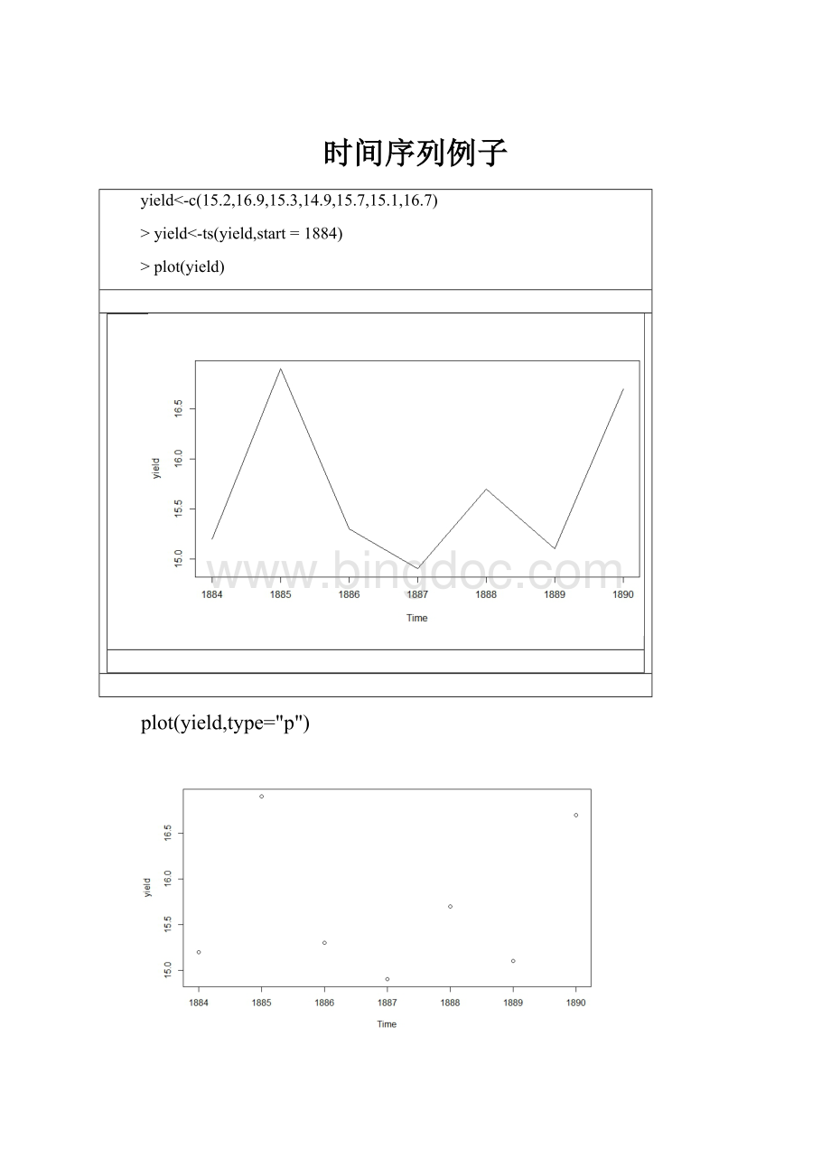
yield<-c（15.2,16.9,15.3,14.9,15.7,15.1,16.7）

>yield<-ts（yield,start=1884）

>plot（yield）

plot（yield,type="p"）

plot（yield,type="o"）

plot（yield,type="h"）

plot（yield,type="o",pch=17）

plot（yield,lty=2）

>plot（yield,lwd=2）

>plot（yield,main='1884-1890',xlab='年份',ylab='产量'）

plot（yield）

>abline（v=1887,lty=2）

>plot（yield）

>abline（v=c（1885,1889）,lty=2）

>plot（yield）

>abline（h=c（15.5,16.5）,lty=2）

>library（TSA）

>data（oil.price）p88石油价格时间序列

>oil.price

JanFebMarAprMayJunJulAugSepOctNovDec

198622.9315.4512.6112.8415.3813.4311.5815.1014.8714.9015.2216.11

198718.6517.7518.3018.6819.4420.0721.3420.3119.5319.8618.8517.27

198817.1316.8016.2017.8617.4216.5315.5015.5214.5413.7714.1416.38

198918.0217.9419.4821.0720.1220.0519.7818.5819.5920.1019.8621.10

199022.8622.1120.3918.4318.2016.7018.4527.3133.5136.0432.3327.28

199125.2320.4819.9020.8321.2320.1921.4021.6921.8923.2322.4619.50

199218.7919.0118.9220.2320.9822.3821.7721.3421.8821.6820.3419.41

199319.0320.0920.3220.2519.9519.0917.8918.0117.5018.1516.6114.51

199415.0314.7814.6816.4217.8919.0619.6518.3817.4517.7218.0717.16

199518.0418.5718.5419.9019.7418.4517.3218.0218.2317.4317.9919.03

199618.8519.0921.3323.5021.1620.4221.3021.9023.9724.8823.7025.23

199725.1322.1820.9719.7020.8219.2619.6619.9519.8021.3220.1918.33

>head（oil.price）

[1]22.9315.4512.6112.8415.3813.43

>tail（oil.price）

[1]64.9865.5962.2658.3259.4165.48

>plot（oil.price）

as.vector（oil.price）

[1]22.9315.4512.6112.8415.3813.4311.5815.1014.8714.9015.2216.1118.6517.7518.3018.6819.4420.0721.34

[20]20.3119.5319.8618.8517.2717.1316.8016.2017.8617.4216.5315.5015.5214.5413.7714.1416.3818.0217.94

[39]19.4821.0720.1220.0519.7818.5819.5920.1019.8621.1022.8622.1120.3918.4318.2016.7018.4527.3133.51

[58]36.0432.3327.2825.2320.4819.9020.8321.2320.1921.4021.6921.8923.2322.4619.5018.7919.0118.9220.23

[77]20.9822.3821.7721.3421.8821.6820.3419.4119.0320.0920.3220.2519.9519.0917.8918.0117.5018.1516.61

[96]14.5115.0314.7814.6816.4217.8919.0619.6518.3817.4517.7218.0717.1618.0418.5718.5419.9019.7418.45

[115]17.3218.0218.2317.4317.9919.0318.8519.0921.3323.5021.1620.4221.3021.9023.9724.8823.7025.2325.13

[134]22.1820.9719.7020.8219.2619.6619.9519.8021.3220.1918.3316.7216.0615.1215.3514.9113.7214.1713.47

[153]15.0314.4613.0011.3512.5112.0114.6817.3117.7217.9220.1021.2823.8022.6925.0026.1027.2629.3729.84

[172]25.7228.7931.8229.7031.2633.8833.1134.4228.4429.5929.6127.2427.4928.6327.6026.4227.3726.2022.17

[191]19.6419.3919.7120.7224.5326.1827.0425.5226.9728.3929.6628.8426.3529.4632.9535.8333.5128.1728.11

[210]30.6630.7531.5728.3130.3431.1132.1334.3134.6836.7436.7540.2738.0240.7844.9045.9453.2848.4743.15

[229]46.8448.1554.1952.9849.8356.3558.9964.9865.5962.2658.3259.4165.48

>acf（as.vector（oil.price）,main='SampleACFoftheOilPriceTimeSeries',xaxp=c（0,24,12））

acf（oil.price,main='SampleACFoftheOilPriceTimeSeries'）

>pacf（as.vector（oil.price）,main='SampleACFoftheOilPriceTimeSeries',xaxp=c（0,24,12））

plot（log（oil.price））

单位根检验

>adf.test（log（oil.price））

AugmentedDickey-FullerTest

data:

log（oil.price）

Dickey-Fuller=-1.1119,Lagorder=6,p-value=0.9189

alternativehypothesis:

stationary

>plot（diff（log（oil.price）））

白噪声检验

>for（iin1:

2）print（Box.test（diff（log（oil.price））,type='Ljung-Box',lag=6*i））

Box-Ljungtest

data:

diff（log（oil.price））

X-squared=18.5959,df=6,p-value=0.004903

Box-Ljungtest

data:

diff（log（oil.price））

X-squared=24.3938,df=12,p-value=0.01797

acf（diff（as.vector（log（oil.price）））,main='SampleACFoftheDifferenceoftheOilPriceTimeSeries',xaxp=c（0,24,12））

>pacf（diff（as.vector（log（oil.price）））,main='SamplePACFoftheDifferenceoftheOilPriceTimeSeries',xaxp=c（0,24,12））

>eacf（diff（log（oil.price）））

AR/MA

012345678910111213

0xooooooooooooo

1xxooooooooxooo

2oxoooooooooooo

3oxoooooooooooo

4oxxooooooooooo

5oxoxoooooooooo

6oxoxoooooooooo

7xxoxoooooooooo

>res=armasubsets（y=diff（log（oil.price））,nar=7,nma=7,

+y.name='test',ar.method='ols'）

>plot（res）

>library（forecast）

>auto.arima（log（oil.price））

Series:

log（oil.price）

ARIMA（0,1,1）

Coefficients:

ma1

0.2956

s.e.0.0693

sigma^2estimatedas0.006717:

loglikelihood=260.29

AIC=-516.58AICc=-516.53BIC=-509.62

条件最小二乘估计

>arima（log（oil.price）,order=c（0,1,1）,method='CSS'）

Call:

arima（x=log（oil.price）,order=c（0,1,1）,method="CSS"）

Coefficients:

ma1

0.2731

s.e.0.0681

sigma^2estimatedas0.006731:

partloglikelihood=259.58

>arima（log（oil.price）,order=c（0,1,1）,method='ML'）

极大似然估计

Call:

arima（x=log（oil.price）,order=c（0,1,1）,method="ML"）

Coefficients:

ma1

0.2956

s.e.0.0693

sigma^2estimatedas0.006689:

loglikelihood=260.29,aic=-518.58

系数的置信区间

>m<-arima（log（oil.price）,order=c（0,1,1）,method='ML'）

>confint（m）

2.5%97.5%

ma10.15968290.4315169

模型诊断

>tsdiag（m）

>tsdiag（m）

>predict（m）

$pred

Feb

20064.20755

$se

Feb

20060.08178378