灰度阀值变换及二值化.docx
《灰度阀值变换及二值化.docx》由会员分享,可在线阅读,更多相关《灰度阀值变换及二值化.docx(9页珍藏版)》请在冰点文库上搜索。
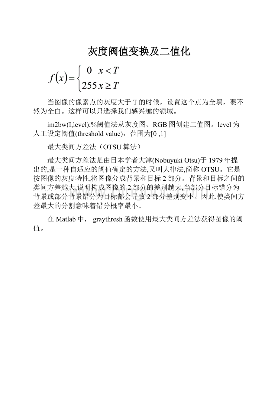
灰度阀值变换及二值化
当图像的像素点的灰度大于T的时候,设置这个点为全黑,要不然为全白。
这样可以只选择我们感兴趣的领域。
im2bw(I,level);%阈值法从灰度图、RGB图创建二值图。
level为人工设定阈值(thresholdvalue),范围为[0,1]
最大类间方差法(OTSU算法)
最大类间方差法是由日本学者大津(NobuyukiOtsu)于1979年提出的,是一种自适应的阈值确定的方法,又叫大律法,简称OTSU。
它是按图像的灰度特性,将图像分成背景和目标2部分。
背景和目标之间的类间方差越大,说明构成图像的2部分的差别越大,当部分目标错分为背景或部分背景错分为目标都会导致2部分差别变小。
因此,使类间方差最大的分割意味着错分概率最小。
在Matlab中, graythresh函数使用最大类间方差法获得图像的阈值。
(注意标点‘‘要换一下)
I=imread(‘beauty_yellowflowers.jpg’);
thresh=graythresh(I);%自适应设置阀值
bw1=im2bw(I,thresh);
bw2=im2bw(I,130/255);%手工设置阀值
subplot(1,3,1);imshow(I);title(‘original’)
subplot(1,3,2);imshow(bw1);title(‘autoset_thresh’);
subplot(1,3,3);imshow(bw2); title(‘thresh=130’);
最小分类错误全局二值化算法(kittlerMet算法)
函数源代码:
functionimagBW=kittlerMet(imag)
%KITTLERMETbinarizesagrayscaleimage'imag'intoabinaryimage
%Input:
% imag:
thegrayscaleimage,withblackforeground(0),andwhite
% background(255).
%Output:
% imagBW:
thebinaryimageofthegrayscaleimage'imag',withkittler's
% minimumerrorthresholdingalgorithm.
%Reference:
% J.KittlerandJ.Illingworth.MinimumErrorThresholding.Pattern
% Recognition.1986.19
(1):
41-47
MAXD=100000;
imag=imag(:
:
1);
[counts,x]=imhist(imag); %countsarethehistogram.xistheintensitylevel.
GradeI=length(x); %theresolusionoftheintensity.i.e.256foruint8.
J_t=zeros(GradeI,1); %criterionfunction
prob=counts./sum(counts); %Probabilitydistribution
meanT=x'*prob; %Totalmeanlevelofthepicture
%Initialization
w0=prob
(1); %Probabilityofthefirstclass
miuK=0; %First-ordercumulativemomentsofthehistogramuptothekthlevel.
J_t
(1)=MAXD;
n=GradeI-1;
fori=1:
n
w0=w0+prob(i+1);
miuK=miuK+i*prob(i+1); %first-ordercumulativemoment
if(w01-eps)
J_t(i+1)=MAXD; %T=i
else
miu1=miuK/w0;
miu2=(meanT-miuK)/(1-w0);
var1=(((0:
i)'-miu1).^2)'*prob(1:
i+1);
var1=var1/w0; %variance
var2=(((i+1:
n)'-miu2).^2)'*prob(i+2:
n+1);
var2=var2/(1-w0);
ifvar1>eps&&var2>eps %incaseofvar1=0orvar2=0
J_t(i+1)=1+w0*log(var1)+(1-w0)*log(var2)-2*w0*log(w0)-2*(1-w0)*log(1-w0);
else
J_t(i+1)=MAXD;
end
end
end
minJ=min(J_t);
index=find(J_t==minJ);
th=mean(index);
th=(th-1)/n
imagBW=im2bw(imag,th);
%figure,imshow(imagBW),title('kittlerbinary');
MATLAB程序:
I=imread('beauty_yellowflowers.jpg');
imagSW=kittlerMet(I);%Kittler算法
bw1=im2bw(I,130/255);%手工设置阀值
subplot(1,3,1);imshow(I);title('original');
subplot(1,3,2);imshow(imagSW);title('kittlerbinary');
subplot(1,3,3);imshow(bw1);title('thresh=130');
结果:
Niblack二值化算法:
Niblack二值化算法是比较简单的局部阈值方法,阈值的计算公式是T=m+k*v,其中m为以该像素点为中心的区域的平均灰度值,v是该区域的标准差,k是一个系数。
matlab程序如下:
I=imread('beauty_yellowflowers.jpg');
I=rgb2gray(I);
w=2;%
max=0;
min=0;
[m,n]=size(I);
T=zeros(m,n);
%
fori=(w+1):
(m-w)
forj=(w+1):
(n-w)
sum=0;
fork=-w:
w
forl=-w:
w
sum=sum+uint32(I(i+k,j+l));
end
end
average=double(sum)/((2*w+1)*(2*w+1));
s=0;
fork=-w:
w
forl=-w:
w
s=s+(uint32(I(i+k,j+l))-average)*(uint32(I(i+k,j+l))-average);
end
end
s=sqrt(double(s)/((2*w+1)*(2*w+1)));
T(i,j)=average+0.2*s;
end
end
fori=1:
m
forj=1:
n
ifI(i,j)>T(i,j)
I(i,j)=uint8(255);
else
I(i,j)=uint8(0);
end
end
end
imshow(I);
此种算法速度很慢,一直都没等到结果,也有可能是程序中有死循环,,费解
改进的算法如下:
(也挺费时间的,效果不好)
I=imread('beauty_yellowflowers.jpg');
I=rgb2gray(I);
[m,n]=size(I);
block=10;
ver=floor(m/block);
hor=floor(n/block);
T=zeros(m,n);
forb_ver=1:
block
forb_hor=1:
block
%T((ver*(b_ver-1)+1):
(ver*b_ver),(hor*(b_hor-1)+1):
(hor*b_hor))=otsu(I((ver*(b_ver-1)+1):
(ver*b_ver),(hor*(b_hor-1)+1):
(hor*b_hor)));
t=0;
fori=(ver*(b_ver-1)+1):
(ver*b_ver)
forj=(hor*(b_hor-1)+1):
(hor*b_hor)
t=t+uint32(I(i,j));
end
end
t=double(t)/(ver*hor);
std_deviation=0;
fori=(ver*(b_ver-1)+1):
(ver*b_ver)
forj=(hor*(b_hor-1)+1):
(hor*b_hor)
std_deviation=std_deviation+(uint32(I(i,j))-t)*(uint32(I(i,j))-t);
end
end
std_deviation=sqrt(double(std_deviation)/(ver*hor));
thr=t+0.2*std_deviation;
fori=(ver*(b_ver-1)+1):
(ver*b_ver)
forj=(hor*(b_hor-1)+1):
(hor*b_hor)
ifI(i,j)>uint8(floor(thr))
T(i,j)=255;
else
T(i,j)=0;
end
end
end
end
end
imshow(T);
效果(不怎么好):
 升级会员
升级会员 