计量经济学第二版第四章答案.docx
《计量经济学第二版第四章答案.docx》由会员分享,可在线阅读,更多相关《计量经济学第二版第四章答案.docx(20页珍藏版)》请在冰点文库上搜索。
计量经济学第二版第四章答案
4.1
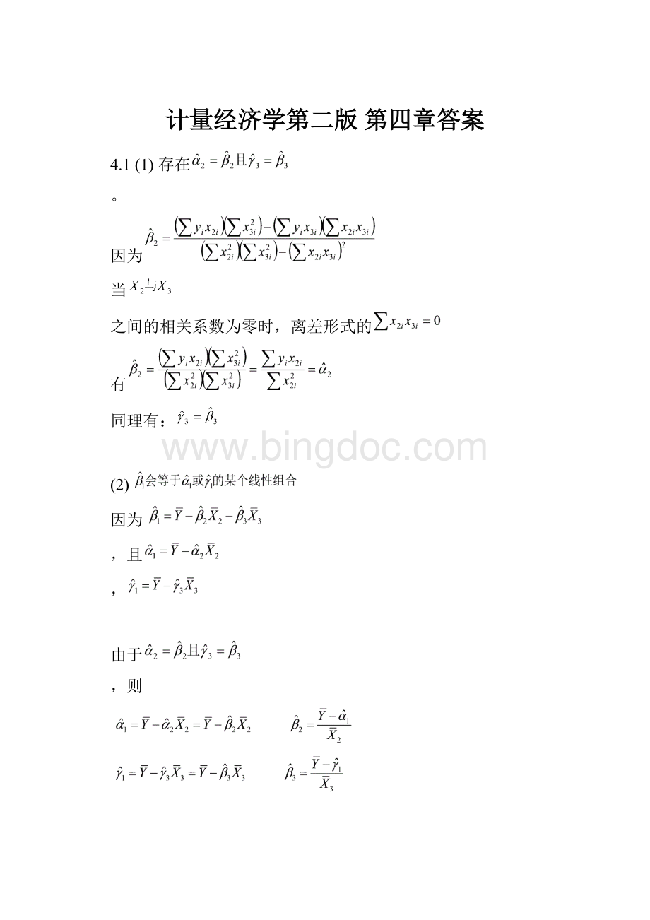
(1)存在
。
因为
当
之间的相关系数为零时,离差形式的
有
同理有:
(2)
因为
,且
,
由于
,则
则
(3)存在
。
因为
当
时,
同理,有
4.3
(1)建立中国商品进口额为Y与国内生产总值x1、居民消费价格指数x2得回归模型
估计模型参数,结果为
DependentVariable:
LNY
Method:
LeastSquares
Date:
05/16/12Time:
19:
15
Sample:
19852007
Includedobservations:
23
Variable
Coefficient
Std.Error
t-Statistic
Prob.
C
-3.060149
0.337427
-9.069059
0.0000
LNX1
1.656674
0.092206
17.96703
0.0000
LNX2
-1.057053
0.214647
-4.924618
0.0001
R-squared
0.992218
Meandependentvar
9.155303
AdjustedR-squared
0.991440
S.D.dependentvar
1.276500
S.E.ofregression
0.118100
Akaikeinfocriterion
-1.313463
Sumsquaredresid
0.278952
Schwarzcriterion
-1.165355
Loglikelihood
18.10482
F-statistic
1275.093
Durbin-Watsonstat
0.745639
Prob(F-statistic)
0.000000
参数估计结果如下:
(2))数据中有多重共线性,居民消费价格指数的回归系数的符号不能进行合理的经济意义解释,且其简单相关系数呈现正向变动。
(3)
DependentVariable:
LNY
Method:
LeastSquares
Date:
05/16/12Time:
19:
17
Sample:
19852007
Includedobservations:
23
Variable
Coefficient
Std.Error
t-Statistic
Prob.
C
-4.090667
0.384252
-10.64579
0.0000
LNX1
1.218573
0.035196
34.62222
0.0000
R-squared
0.982783
Meandependentvar
9.155303
AdjustedR-squared
0.981963
S.D.dependentvar
1.276500
S.E.ofregression
0.171438
Akaikeinfocriterion
-0.606254
Sumsquaredresid
0.617208
Schwarzcriterion
-0.507515
Loglikelihood
8.971921
F-statistic
1198.698
Durbin-Watsonstat
0.364369
Prob(F-statistic)
0.000000
DependentVariable:
LNY
Method:
LeastSquares
Date:
05/16/12Time:
19:
18
Sample:
19852007
Includedobservations:
23
Variable
Coefficient
Std.Error
t-Statistic
Prob.
C
-5.442420
1.253662
-4.341218
0.0003
LNX2
2.663790
0.228046
11.68091
0.0000
R-squared
0.866619
Meandependentvar
9.155303
AdjustedR-squared
0.860268
S.D.dependentvar
1.276500
S.E.ofregression
0.477166
Akaikeinfocriterion
1.441037
Sumsquaredresid
4.781435
Schwarzcriterion
1.539775
Loglikelihood
-14.57192
F-statistic
136.4437
Durbin-Watsonstat
0.152312
Prob(F-statistic)
0.000000
DependentVariable:
LNX1
Method:
LeastSquares
Date:
05/16/12Time:
19:
19
Sample:
19852007
Includedobservations:
23
Variable
Coefficient
Std.Error
t-Statistic
Prob.
C
-1.437984
0.734328
-1.958231
0.0636
LNX2
2.245971
0.133577
16.81400
0.0000
R-squared
0.930855
Meandependentvar
10.87007
AdjustedR-squared
0.927563
S.D.dependentvar
1.038480
S.E.ofregression
0.279498
Akaikeinfocriterion
0.371300
Sumsquaredresid
1.640506
Schwarzcriterion
0.470039
Loglikelihood
-2.269955
F-statistic
282.7107
Durbin-Watsonstat
0.142984
Prob(F-statistic)
0.000000
单方程拟合效果都很好,回归系数显著,可决系数较高,GDP和CPI对进口分别有显著的单一影响,在这两个变量同时引入模型时影响方向发生了改变;GDP对CPI进行回归分析,回归系数显著,判定系数较高,说明GDP和CPI有很强的线性关系,这正是原模型多重共线性的原因。
(4)如果仅仅是作预测,可以不在意这种多重共线性,但如果是进行结构分析,还是应该引起注意。
4.6
(1)建立对数线性多元回归模型,引入全部变量建立对数线性多元回归模型如下:
变量对数线性多元回归,结果为:
DependentVariable:
LNY
Method:
LeastSquares
Date:
05/16/12Time:
19:
29
Sample:
19852007
Includedobservations:
23
Variable
Coefficient
Std.Error
t-Statistic
Prob.
C
3.442051
2.706112
1.271954
0.2228
LNX1
11.83820
2.309722
5.125377
0.0001
LNX2
-11.33780
1.932927
-5.865609
0.0000
LNX3
-0.371450
0.719447
-0.516300
0.6132
LNX4
0.219891
0.152083
1.445857
0.1688
LNX5
-0.182164
0.105332
-1.729434
0.1042
LNX6
0.225508
0.302923
0.744439
0.4681
LNX7
1.270052
0.484728
2.620134
0.0193
R-squared
0.993930
Meandependentvar
11.78641
AdjustedR-squared
0.991097
S.D.dependentvar
0.343125
S.E.ofregression
0.032375
Akaikeinfocriterion
-3.754629
Sumsquaredresid
0.015722
Schwarzcriterion
-3.359675
Loglikelihood
51.17824
F-statistic
350.8771
Durbin-Watsonstat
1.539809
Prob(F-statistic)
0.000000
从修正的可决系数和F统计量可以看出,全部变量对数线性多元回归整体对样本拟合很好,,各变量联合起来对能源消费影响显著。
可是其中的lnX4、lnX6对lnY影响不显著,而且lnX2、lnX3、lnX5的参数为负值,在经济意义上不合理。
所以这样的回归结果并不理想。
(2)解释变量国民总收入(亿元)X1(代表收入水平)、国内生产总值(亿元)X2(代表经济发展水平)、工业增加值(亿元)X3、建筑业增加值(亿元)X4、交通运输邮电业增加值(亿元)X5(代表产业发展水平及产业结构)、人均生活电力消费(千瓦小时)X6(代表人民生活水平提高)、能源加工转换效率(%)X7(代表能源转换技术)等很可能线性相关,计算相关系数如下
变量
LNX1
LNX2
LNX3
LNX4
LNX5
LNX6
LNX7
LNX1
1
0.999974
0.999733
0.996913
0.993576
0.99717
0.708415
LNX2
0.999974
1
0.999746
0.997177
0.993839
0.996819
0.709065
LNX3
0.999733
0.999746
1
0.997887
0.991701
0.995511
0.71606
LNX4
0.996913
0.997177
0.997887
1
0.989591
0.989932
0.708962
LNX5
0.993576
0.993839
0.991701
0.989591
1
0.993937
0.664793
LNX6
0.99717
0.996819
0.995511
0.989932
0.993937
1
0.685726
LNX7
0.708415
0.709065
0.71606
0.708962
0.664793
0.685726
1
可以看出lnx1与lnx2、lnx3、lnx4、lnx5、lnx6之间高度相关,许多相关系数高于0.900以上。
如果决定用表中全部变量作为解释变量,很可能会出现严重多重共线性问题。
(3)因为存在多重共线性,解决方法如下:
DependentVariable:
Y
Method:
LeastSquares
Date:
05/16/12Time:
19:
49
Sample:
19852007
Includedobservations:
23
Variable
Coefficient
Std.Error
t-Statistic
Prob.
C
-76917.33
103078.4
-0.746202
0.4671
X1
15.23223
4.658786
3.269570
0.0052
X2
-15.90504
4.478372
-3.551523
0.0029
X3
-2.633378
3.649937
-0.721486
0.4817
X4
26.26439
11.12634
2.360561
0.0322
X5
0.074759
3.675204
0.020341
0.9840
X6
890.4204
364.5072
2.442806
0.0274
X7
2155.185
1498.804
1.437937
0.1710
R-squared
0.989342
Meandependentvar
139423.9
AdjustedR-squared
0.984368
S.D.dependentvar
51806.33
S.E.ofregression
6477.323
Akaikeinfocriterion
20.65821
Sumsquaredresid
6.29E+08
Schwarzcriterion
21.05316
Loglikelihood
-229.5694
F-statistic
198.9049
Durbin-Watsonstat
1.278853
Prob(F-statistic)
0.000000
由图可以看出还是有严重多重共线性。
我会采用逐步回归的办法,去检验和解决多重共线性问题:
DependentVariable:
Y
Method:
LeastSquares
Date:
05/16/12Time:
19:
59
Sample:
19852007
Includedobservations:
23
Variable
Coefficient
Std.Error
t-Statistic
Prob.
C
79949.57
2951.120
27.09126
0.0000
X1
0.734487
0.027916
26.31049
0.0000
R-squared
0.970557
Meandependentvar
139423.9
AdjustedR-squared
0.969155
S.D.dependentvar
51806.33
S.E.ofregression
9098.624
Akaikeinfocriterion
21.15258
Sumsquaredresid
1.74E+09
Schwarzcriterion
21.25131
Loglikelihood
-241.2546
F-statistic
692.2419
Durbin-Watsonstat
0.317238
Prob(F-statistic)
0.000000
DependentVariable:
Y
Method:
LeastSquares
Date:
05/16/12Time:
19:
57
Sample:
19852007
Includedobservations:
23
Variable
Coefficient
Std.Error
t-Statistic
Prob.
C
79577.18
3085.516
25.79056
0.0000
X2
0.736521
0.029176
25.24391
0.0000
R-squared
0.968097
Meandependentvar
139423.9
AdjustedR-squared
0.966578
S.D.dependentvar
51806.33
S.E.ofregression
9471.027
Akaikeinfocriterion
21.23280
Sumsquaredresid
1.88E+09
Schwarzcriterion
21.33154
Loglikelihood
-242.1772
F-statistic
637.2550
Durbin-Watsonstat
0.303167
Prob(F-statistic)
0.000000
DependentVariable:
Y
Method:
LeastSquares
Date:
05/16/12Time:
19:
59
Sample:
19852007
Includedobservations:
23
Variable
Coefficient
Std.Error
t-Statistic
Prob.
C
81615.09
2696.634
30.26555
0.0000
X3
1.733167
0.061139
28.34793
0.0000
R-squared
0.974533
Meandependentvar
139423.9
AdjustedR-squared
0.973321
S.D.dependentvar
51806.33
S.E.ofregression
8461.964
Akaikeinfocriterion
21.00749
Sumsquaredresid
1.50E+09
Schwarzcriterion
21.10623
Loglikelihood
-239.5862
F-statistic
803.6049
Durbin-Watsonstat
0.331246
Prob(F-statistic)
0.000000
DependentVariable:
Y
Method:
LeastSquares
Date:
05/16/12Time:
19:
59
Sample:
19852007
Includedobservations:
23
Variable
Coefficient
Std.Error
t-Statistic
Prob.
C
79251.87
3030.263
26.15346
0.0000
X4
13.21408
0.512296
25.79385
0.0000
R-squared
0.969402
Meandependentvar
139423.9
AdjustedR-squared
0.967945
S.D.dependentvar
51806.33
S.E.ofregression
9275.342
Akaikeinfocriterion
21.19105
Sumsquaredresid
1.81E+09
Schwarzcriterion
21.28979
Loglikelihood
-241.6971
F-statistic
665.3228
Durbin-Watsonstat
0.314072
Prob(F-statistic)
0.000000
DependentVariable:
Y
Method:
LeastSquares
Date:
05/16/12Time:
20:
00
Sample:
19852007
Includedobservations:
23
Variable
Coefficient
Std.Error
t-Statistic
Prob.
C
82253.98
5537.916
14.85288
0.0000
X5
10.92177
0.810459
13.47603
0.0000
R-squared
0.896349
Meandependentvar
139423.9
AdjustedR-squared
0.891414
S.D.dependentvar
51806.33
S.E.ofregression
17071.46
Akaikeinfocriterion
22.41115
Sumsquaredresid
6.12E+09
Schwarzcriterion
22.50988
Loglikelihood
-255.7282
F-statistic
181.6035
Durbin-Watsonstat
0.382638
Prob(F-statistic)
0.000000
DependentVariable:
Y
Method:
LeastSquares
Date:
05/16/12Time:
20:
00
Sample:
19852007
Includedobservations:
23
Variable
Coefficient
Std.Error
t-Statistic
Prob.
C
66876.70
3935.724
16.99222
0.0000
X6
679.2253
30.41199
22.33413
0.0000
R-squared
0.959601
Meandependentvar
139423.9
AdjustedR-squared
0.957677
S.D.dependentvar
51806.33
S.E.ofregression
10657.87
Akaikeinfocriterion
21.46893
Sumsquaredresid
2.39E+09
Schwarzcriterion
21.56766
Loglikelihood
-244.8926
F-statistic
498.8135
Durbin-Watsonstat
0.291768
Prob(F-statistic)
0.000000
DependentVariable:
Y
Method:
LeastSquares
Date:
05/16/12Time:
20:
00
Sample:
19852007
Includedobservations:
23
Variable
Coefficient
Std.Error
t-Statistic
Prob.
C
-1191355.
283030.8
-4.209278
0.0004
X7
19372.59
4118.642
4.703636
0.0001
R-squared
0.513034
Meandependentvar
139423.9
AdjustedR-squared
0.489846
S.D.dependentvar
51806.33
S.E.ofregression
37002.72
Akaikeinfocriterion
23.95831
Sumsquared
 升级会员
升级会员 