东南大学matlab大作业第二次.docx
《东南大学matlab大作业第二次.docx》由会员分享,可在线阅读,更多相关《东南大学matlab大作业第二次.docx(33页珍藏版)》请在冰点文库上搜索。
东南大学matlab大作业第二次
MatlabWorksheet2
PartA(In-classroomexercises)
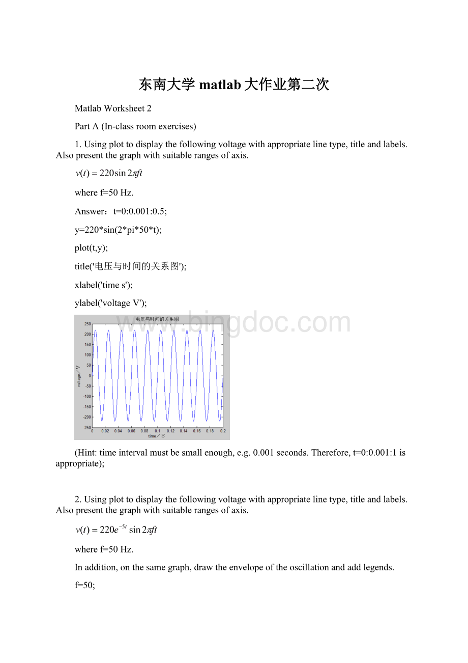
1.Usingplottodisplaythefollowingvoltagewithappropriatelinetype,titleandlabels.Alsopresentthegraphwithsuitablerangesofaxis.
wheref=50Hz.
Answer:
t=0:
0.001:
0.5;
y=220*sin(2*pi*50*t);
plot(t,y);
title('电压与时间的关系图');
xlabel('times');
ylabel('voltageV');
(Hint:
timeintervalmustbesmallenough,e.g.0.001seconds.Therefore,t=0:
0.001:
1isappropriate);
2.Usingplottodisplaythefollowingvoltagewithappropriatelinetype,titleandlabels.Alsopresentthegraphwithsuitablerangesofaxis.
wheref=50Hz.
Inaddition,onthesamegraph,drawtheenvelopeoftheoscillationandaddlegends.
f=50;
t=0:
0.001:
1;
v1=220*exp(-5*t).*sin(2*pi*f*t);
plot(t,v1,'g','LineWidth',4)
axis([00.1-220220])
holdon;
v2=220*exp(-5*t);
plot(t,v2,'r--','LineWidth',2);
holdoff;
holdon;
v2=-220*exp(-5*t);
plot(t,v2,'r--','LineWidth',2);
xlabel('time(s)'),ylabel('voltage(V)'),title('VoltageAgainstTime')
legend('v1','v2',2);
holdoff;
3.Usesubplot,drawa2by2arrayofplotsforthefollowingfunctions:
Applyappropriatelinetype,title,labelsandaxisrangesforthegraphs.
t=0:
0.001:
1;
subplot(221),plot(t,cos(10*pi*t))
xlabel('t'),ylabel('cos(10*pi*t)')
subplot(222),plot(t,cos(10*pi*t).*exp(-5*t))
xlabel('t'),ylabel('cos(10*pi*t).*exp(-5*t)')
subplot(223),plot(t,cos(10*pi*t).*exp(-10*t))
xlabel('t'),ylabel('cos(10*pi*t).*exp(-10*t)')
subplot(224),plot(t,cos(10*pi*t).*exp(-20*t))
xlabel('t'),ylabel('cos(10*pi*t).*exp(-20*t)')
4.Useplot3toplot2spiralcurveslikebelowwithappropriatelinewidthandcolour.
t=0:
0.01:
10;
x=0.02*t.^2.*sin(2*pi*t);
y=0.02*t.^2.*cos(2*pi*t);
z=0.2*t;
subplot(121),plot3(x,y,z,'g','LineWidth',1);
axis([-22-2202]);
gridon;
%holdon;
t=0:
0.01:
10;
x=0.7*t.^0.4.*sin(2*pi*t);
y=0.7*t.^0.4.*cos(2*pi*t);
z=0.2*t;
subplot(122),plot3(x,y,z,'r','LineWidth',1);
axis([-22-2202]);
gridon;
%holdoff;
5.Displaythesurfaceusingmeshandcontourwithasuitableresolution(分辨率):
[x,y]=meshgrid(1:
0.1:
100,1:
0.1:
100);
f=exp(-0.005.*((x-50).^2+(y-50).^2));
figure
(1)
mesh(x,y,f),xlabel('x'),ylabel('y'),gridon;
figure
(2),contour(x,y,f)
xlabel('x'),ylabel('y'),grid;
6.Load2ofyourphotosintoMatlabWorkSpaceusingimread.a)Changebrightnesslocallyorglobally.b)Overlapthemtoproduceanewphoto.c)writeanewphotointoafileusingimwrite.(Note:
lowerversionofMatlabsuchas6.5isnotallowedtodosomedirectimageoperations.)
A=imread('hw1.jpg');
B=imread('hw2.jpg');
figure
(1),imshow(A);
figure
(2),imshow(B);
size(A);
%figure
(2),histeq(A(:
:
1))
figure(3),imshow(A+100);
[m,n,l]=size(A);
C(1:
m,1:
n,1:
l)=B(1:
m,1:
n,1:
l);
figure(4),imshow(A+C);
imwrite(A+C,'hw4.bmp',’bmp’);
7.Forlinearsimultaneousequations
theequationcoefficients:
A=[1-143
-545-6
07-89
-13-26];(M=N)
a)FindthedeterminantofA,行列式
b)Findtheinverse(倒数)ofAandcheckformatrixsingularity,
c)IfB=[5;1;-2;3],findtheunknownxintheequation.
A=[1-143;-545-6;07-89;-13-26];
B=[5;1;-2;3];
x=inv(A)*B
det(A)
cond(A)%计算A的条件数
x=
-1.0000
-0.5882
0.7059
0.8627
ans=
-765.0000
ans=
16.4186
Sonotsingular
8.Forlinearsimultaneousequations,(线性联立方程)
M>N,theequationcoefficients:
A=[1-143
-545-6
07-89
-13-26
1-253
147-3];
a)FindthedeterminantofA’*A,
b)FindtheinverseofA’*Aandcheckformatrixsingularity,
c)IfB=[5;1;-2;3;4;0],findthesolutionoftheequation.
A=[1-143;-545-6;07-89;-13-26;1-253;047-3];
B=[5;1;-2;3;4;0];
x=A\B
x=inv(A'*A)*A'*B
det(A'*A)
cond(A'*A)%乘以A’
x=
-0.8903
-0.4898
0.5755
0.7083
x=
-0.8903
-0.4898
0.5755
0.7083
ans=
2.1051e+07
ans=
32.5278
Notsingular
9.Dataof10recordsareshownbelow
y=[3.54.33.75.46.67.38.78.89.49.010.012.011.39.913.3],
Usepolyfitwithdifferentorders(from1to3)ofpolynomialstofindacurveofbestfit.Checkthetotaldistancebetweenthefittedcurvezandrecordsdefinedby
.
%createacurvewithnoise
clearall;
closeall;
x=0:
1:
14;
y=[3.54.33.75.46.67.38.78.89.49.010.012.011.39.913.3]
plot(x,y,'x');
holdon;
%curvefittedbya
%2ndorderpolynomial
p=polyfit(x,y,3);
z=polyval(p,x);
plot(x,z,'r','LineWidth',2);
holdoff;
gridon;
s=sqrt(sum((z-y).^2))
10.Createasetof20pointsfromacurvebyMatlabcode:
x=1:
20;y=2*exp(-0.3*(x-5).^2)+0.7*exp(-0.2*(x-12).^2);
Theninterpolatethecurveto60pointsusing‘linear’and‘spline’options,respectively.Seethequalityofdifferenttypesofinterpolation.(插值法)
x=1:
20;y=2*exp(-0.3*(x-5).^2)+0.7*exp(-0.2*(x-12).^2);
xi=linspace(1,20,60);
yi=interp1(x,y,xi,'linear');
plot(x,y,'g*');holdon;
plot(xi,yi,'ro');
plot(xi,yi,':
');
holdon;
x=1:
20;y=2*exp(-0.3*(x-5).^2)+0.7*exp(-0.2*(x-12).^2);
xi=linspace(1,20,60);
yi=interp1(x,y,xi,'spline');
plot(x,y,'yx');holdon;
plot(xi,yi,'o');
plot(xi,yi,':
');
holdoff;
PartB
1.Usingtheplotandsubplotfunctionscreate4plotsona2by2arrayofsubplots,forthefunctionexp(-t)sin(5t)showingineachplotthefunctioninthecorrespondingintervalsofti.e.(-2,-1),(-1,0),(0,1)and(1,2).
Answer:
t=-2:
0.001:
-1;
subplot(221),plot(t,exp(t).*sin(5*t))
xlabel('t'),ylabel('exp(t).*sin(5*t)')
t=-1:
0.001:
0;
subplot(222),plot(t,exp(t).*sin(5*t))
xlabel('t'),ylabel('exp(t).*sin(5*t)')
t=0:
0.001:
1;
subplot(223),plot(t,exp(t).*sin(5*t))
xlabel('t'),ylabel('exp(t).*sin(5*t)')
t=1:
0.001:
2;
subplot(224),plot(t,exp(t).*sin(5*t))
xlabel('t'),ylabel('exp(t).*sin(5*t)')
2.Athreephaseinductionmotorcharacteristic(三相电机特性)isgivenintermsofmechanicalshaftoutputtorque
(NMNewton-meter)asafunctionofrotationalspeedω(rad/sradianpersecond).Thisisapproximatedby3piece-wiselinearequationsasfollows:
Thismotorisdirectlycoupledtoaload
whichcanberepresentedas
Write2separateMatlabfunctionm-filesinwhich:
a)themotorcharacteristic,b)theloadcharacteristicaredefinedonlyasfunctionsofω.Namethemmotor.mandsysload.m,respectively.
Answer:
a)functiony=motor(w)
ifw>=0&&w<90*pi
y=w/(90*pi)+4.0;
elseifw>=90*pi&&w<110*pi
y=95*w/(20*pi)-422.5;
elseifw>=110*pi&&w<=120*pi
y=-10*w/pi+1200;
end
end
end
b)
functiony=sysload(w)
y=-50*(w/(120*pi))^3+100*(w/(120*pi))^2+4*w/(120*pi);
end
3.WriteaMatlabscripgt-mfilewhichcallsyourfunctionm-filesfromQuestion2.Andplotthemotorandloadcharactersticsonthesamefigure,givingsuitablelabellingandtitle.Namethisscriptm-filesystemplot.m
Answer:
x=0:
0.01:
120*pi;
l=length(x);
y=zeros(1,l);
z=zeros(1,l);
fori=1:
l
y(i)=motor1(x(i));
z(i)=sysload1(x(i));
end
plot(x,y,'r',x,z,'g','linewidth',2);
title('MotorandLoadcharacteristics');
legend('MotorCharacteristic','LoadCharacteristic',2);
4.Writeasriptm-filewhichfindsallthemathematicallpossiblepoints(valuesofω)where
5.
fortherange0≤ω≤120π(rad/s)withthecharacteristicgiveninQuestion2.Thesystemcouldtheoreticallyoperateataspeedωwhere
Mathematically,thisinvolvesfindingtherootsoftheequation
Giveanametothism-fileposspoints.m.Callposspoints.minsystemplot.mandshowallofthepointsonasystemplotusingthe‘o’symbol.
%systemplot.m
symsxyz;
y=motor(x);
z=sysload(x);
a=ezplot(y,[0,120*pi]);
holdon;
b=ezplot(z,[0,120*pi]);
set(a,'color','r','linewidth',2);
set(b,'color','g','linewidth',2);
axistight;
title('MotorandLoadcharacteristics');
legend('MotorCharacteristic','LoadCharacteristic',2);
holdon;
[out_x,out_y]=possiblepoints();
plot(out_x,out_y,'o');
%posspoints.m
function[out_x,out_y]=possiblepoints()
symsxyzg;
y=motor(x);
z=sysload(x);
g=y-z;
k=solve(g);
out_x=zeros(1,3);
out_y=zeros(1,3);
fori=3:
5
out_x(i)=double(k(i));
out_y(i)=motor(out_x(i));
end
end
functiony=motor(varargin)
ifstrcmp(class(varargin{1}),'double')==1%±È½Ï×Ö·û´®
w=varargin{1};
ifw>=0&&w<90*pi
y=w/(90*pi)+4.0;
elseifw>=90*pi&&w<110*pi
y=95*w/(20*pi)-422.5;
elseifw>=110*pi&&w<=120*pi
y=-10*w/pi+1200;
end
end
end
else
symsx;
y=(x/(90*pi)+4.0)*(heaviside(x)-heaviside(x-90*pi))+(95*x/(20*pi)-422.5)*(heaviside(x-90*pi)-heaviside(x-110*pi))+(-10*x/pi+1200)*(heaviside(x-110*pi)-heaviside(x-120*pi));
end
end
functiony=sysload(varargin)
symsx;
ifstrcmp(class(varargin{1}),'double')==1
w=varargin{1};
y=-50*(w/(120*pi))^3+100*(w/(120*pi))^2+4*w/(120*pi);
else
y=-50*(x/(120*pi))^3+100*(x/(120*pi))^2+4*x/(120*pi);
end
Answer:
w=(0:
0.1:
120)*pi;
%count=0;
a=1;
fori=1:
1201
z1(i)=motor(w(i));
z2(i)=sysload(w(i));
end
fori=2:
1201;
if((z1(i)-z2(i))*(z1(i-1)-z2(i-1)))<=0
%count=count+1;
r(a)=w(i);
z3(a)=motor(r(a));
a=a+1;
%if(z1(i)-z2(i))==0;
%count=count-1;
%end
end
end
r
plot(r,z3,'o');
%systomplot
w=(0:
0.1:
120)*pi;
fori=1:
1201
y1(i)=motor(w(i));
y2(i)=sysload(w(i));
end
plot(w,y1,'b');
holdon;
plot(w,y2,'r');holdon;
legend('TM','TL',2);
xlabel('w');
ylabel('TL&TM');
title('systemplot');
posspoints;
PartC
IntroductiontoDSP
1.Basicdigitalsignals
Unitimpulsefunction
Exercise1-1:
DisplaytheunitimpulsefunctionwithMatlabcode.ThecodecanbeeithertypedunderMatlabpromptorwrittenintoascriptMatlabfile,thenrunthefile.
n=-10:
10;
fork=1:
21
x(k)=0;
end;
x(11)=1;
stem(n,x);
axis([-101002]);
Problem1-1:
Forthesignal
writetheMatlabcodeandcopytheresultfigureintothefollowingboxe
 升级会员
升级会员 