实验四 信号与系统的复频域分析.docx

实验四 信号与系统的复频域分析.docx

《实验四 信号与系统的复频域分析.docx》由会员分享，可在线阅读，更多相关《实验四 信号与系统的复频域分析.docx（13页珍藏版）》请在冰点文库上搜索。

实验四信号与系统的复频域分析

实验四信号与系统的复频域分析

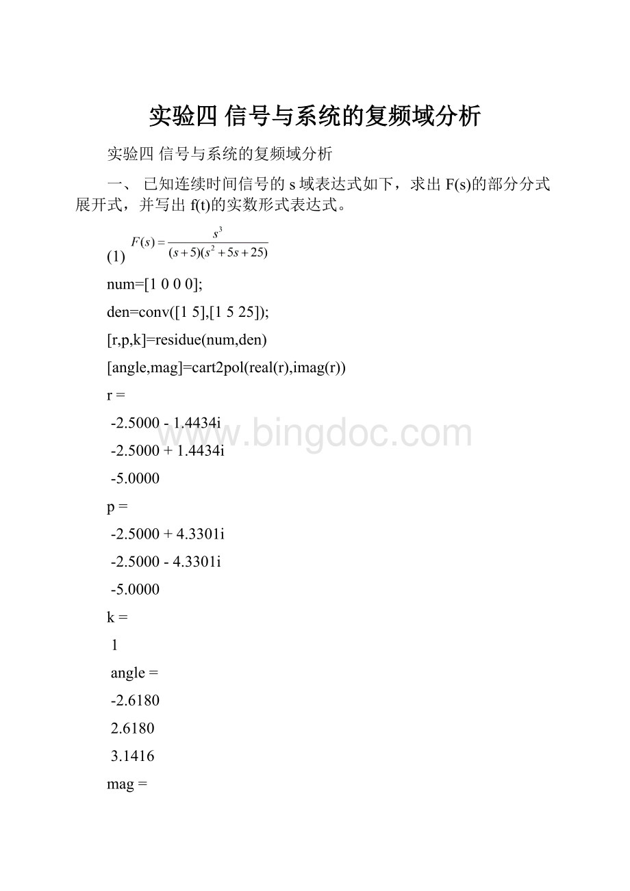
一、已知连续时间信号的s域表达式如下，求出F（s）的部分分式展开式，并写出f（t）的实数形式表达式。

（1）

num=[1000];

den=conv（[15],[1525]）;

[r,p,k]=residue（num,den）

[angle,mag]=cart2pol（real（r）,imag（r））

r=

-2.5000-1.4434i

-2.5000+1.4434i

-5.0000

p=

-2.5000+4.3301i

-2.5000-4.3301i

-5.0000

k=

1

angle=

-2.6180

2.6180

3.1416

mag=

2.8868

2.8868

5.0000

（2）

num=[833.3025];

den=conv（[14.112328.867],[19.927928.867]）;

[r,p]=residue（num,den）

[angle,mag]=cart2pol（real（r）,imag（r））

r=

2.4819-5.9928i

2.4819+5.9928i

-2.4819+1.0281i

-2.4819-1.0281i

p=

-4.9640+2.0558i

-4.9640-2.0558i

-2.0562+4.9638i

-2.0562-4.9638i

angle=

-1.1782

1.1782

2.7489

-2.7489

mag=

6.4864

6.4864

2.6864

2.6864

二、归一化的Butterworth滤波器的系统函数为

。

（1）求出H（s）的部分分式展开式，并写出h（t）的实数形式表达式；

num=[1];

den=conv（[12*sin（pi/8）1],[12*sin（3*pi/8）1]）;

[r,p]=residue（num,den）

[angle,mag]=cart2pol（real（r）,imag（r））

r=

-0.4619+0.1913i

-0.4619-0.1913i

0.4619-1.1152i

0.4619+1.1152i

p=

-0.3827+0.9239i

-0.3827-0.9239i

-0.9239+0.3827i

-0.9239-0.3827i

angle=

2.7489

-2.7489

-1.1781

1.1781

mag=

0.5000

0.5000

1.2071

1.2071

（2）用impulse求出其h（t），并和

（1）中的结果进行比较。

num=[1];

den=conv（[12*sin（pi/8）1],[12*sin（3*pi/8）1]）;

sys=tf（num,den）;

t=0:

0.02:

10;

h=impulse（sys,t）;

plot（t,h）;

title（'ImpulseResponse'）

三、已知信号系统函数

，试分别画出

时系统的零极点图。

如果系统是稳定的，画出系统的幅度响应曲线。

系统极点的位置对系统幅度响应有何影响？

程序：

a=input（'a='）;

num=[1];

den=[12*a1];

sys=tf（num,den）;

poles=roots（den）

pzmap（sys）;

（1）系统不是稳定的

a=0F（s）=1/（s^2+1）

num=[1];

den=[101];

sys=tf（num,den）;

poles=roots（den）

pzmap（sys）;

poles=

0+1.0000i

0-1.0000i

（2）系统是稳定的

a=1/4F（s）=1/（s^2+1/2*s+1）

num=[1];

den=[11/21];

sys=tf（num,den）;

poles=roots（den）

figure

（1）;pzmap（sys）;

w=linspace（0,5,200）;

F=freqs（num,den,w）;

figure

（2）;plot（w,abs（F））;

poles=

-0.2500+0.9682i

-0.2500-0.9682i

（3）系统是稳定的

a=1

num=[1];

den=[121];

sys=tf（num,den）;

poles=roots（den）

figure

（1）;pzmap（sys）;

w=linspace（0,5,200）;

F=freqs（num,den,w）;

figure

（2）;plot（w,abs（F））;

poles=

-1

-1

（4）系统是稳定的

a=2

num=[1];

den=[141];

sys=tf（num,den）;

poles=roots（den）

figure

（1）;pzmap（sys）;

w=linspace（0,5,200）;

F=freqs（num,den,w）;

figure

（2）;plot（w,abs（F））;

poles=

-3.7321

-0.2679

四、已知

，画出该系统的零极点分布图，求出系统的冲激响应、阶跃响应和频率响应。

num=[12];

den=[1221];

sys=tf（num,den）;

poles=roots（den）

figure

（1）;pzmap（sys）;

t=0:

0.02:

10;

h=impulse（num,den,t）;

figure

（2）;plot（t,h）;

title（'ImpulseResponse'）

t=0:

0.02:

10;

s=step（num,den,t）;

figure（3）;plot（t,s）;

title（'StepResponse'）

[H,w]=freqs（num,den）;

figure（4）;plot（w,abs（H））;

xlabel（'\omega'）

title（'MagnitadeResponse'）

poles=

-1.0000

-0.5000+0.8660i

-0.5000-0.8660i